This blog post looks at closed-hand Chinese Poker, and describes a near-optimal strategy for it which is readily implementable on a computer.
Chinese Poker is a 2-4 player gambling card game where each player gets dealt thirteen cards, and then secretly arranges them into three poker hands: the “back” and “middle” of five cards each, and the “front” of three cards. The back hand must be stronger than the middle hand which must be stronger than the front hand.
Once each player has arranged their hands, everyone reveals the arrangement of their cards. Scoring is done between every pair of players. There’s different variants, but in this article we’ll assume that 1 point is scored for each of front, middle and back that beats the corresponding hand in the other player’s board, and an extra 1 point if you beat the player on more hands than you lost. This way of scoring is called 4-2 scoring because assuming no ties either one player beats the other player on all three hands (scoring 4 = 1+1+1 plus 1 for the majority), or one player beats the other player on two out of three hands (scoring 2 = 1+1-1 plus 1 for the majority).
To give an example, let’s suppose Alice and Bob are playing for $10 per point.
Alice gets dealt: 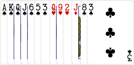
Bob gets dealt: 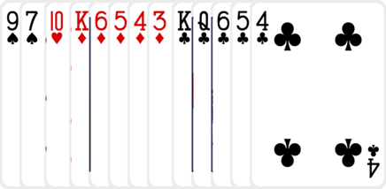
Without seeing each other’s hands, Alice and Bob arrange their cards into back, middle and front hands.
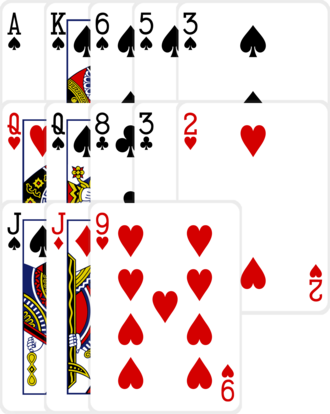
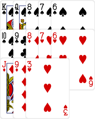
Alice arranges her hand like this:
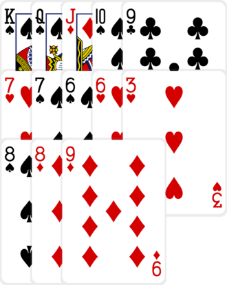
Bob arranges his hand like this:
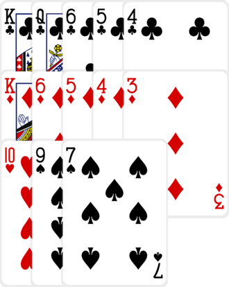
Alice beats Bob in the back hand (Ace-high flush beats King-high flush), loses to Bob in the middle hand (a pair of Queens loses to a King-high flush), and beats Bob in the front hand (a pair of Jacks beats Ten-high).
Alice wins 1 point each for front and back, loses 1 for the middle, and gains 1 for winning the majority for a total of 2 points. Bob pays Alice $20 and the hand is over.
We can see some interesting strategy: Alice chose to have a weak middle hand of a pair of Queens (which is relatively unlikely to win), which allowed her to put a pair of Jacks in the front (which is relatively likely to win there). This paid off for her, allowing her to make a profit with an overall weak hand.
Optimal Counter-Strategy
For a given opponent (with a known strategy) we can find the best counter-strategy. Suppose Alice has been dealt her hand and wants to arrange them to maximize her expected value against Bob. She can mentally deal out many potential hands for Bob and see how he plays them (which she can do because she has perfect knowledge of Bob’s strategy). Then she can pick the arrangement of her own cards to score as high (on average) as possible. Apart from the large amount of computation this entails, it’s relatively simple to implement.
In practice, we don’t know our opponent’s strategy, but we can use this idea as a way to bootstrap a strategy that plays well. The obvious idea is to start with some strategy, construct it’s optimal counter-strategy, then the optimal counter-counter-strategy and so on. If $S_0$ is an initial strategy and $C(S)$ is its optimal counter-strategy then we can construct a sequence of (hopefully improving) strategies like this:
$$S_n = C(S_{n-1})$$
In general this doesn’t work because strategies tend to oscillate. For example, if we try to learn to play optimal rock-paper-scissors and start with the strategy of “always play rock”, then the optimal counter-strategy is “always play paper”, and the optimal counter-counter-strategy is “always play scissors”, and the optimal counter-counter-counter-strategy is back to “always play rock”. A fix to this is to use a blended strategy.
$$S_n = \mathrm{blend}(C(S_{n-1}), S_{n-1})$$
One interpretation is to blend the strategies by non-deterministically choosing between them for each decision. This (for specific weights of the non-deterministic choice) was proven to converge to an optimal strategy in An iterative method of solving a game, Julia Robinson (1950).
The approach I’ll take will be similar but not identical to that idea, but the result will be the same: the sequence will converge to a near-optimal (only slightly exploitable) strategy.
Parameterizing the Strategy
To define our strategy, we’ll define a scoring function that takes a triple (front, middle, back) of hands and returns an expected value. Our computer player, given a hand of 13 cards, will then pick the arrangement that maximizes the score.
Since there’s a lot of triples of hands, I tried an experiment of factoring the scoring algorithm into three parts. The idea here is to estimate a probability that each part of the hand would win independently of the other parts of the hand. For example, a strategy might think AA2 in the front has 95% chance of winning against a good opponent. Then, given the three probabilities $p_f, p_m, p_b$ which correspond to the probabilities that the front, middle and back hands win, the program can compute the expectation for the score. I was surprised to find that there’s relatively few unique hands: for the 5-card middle and back hands there’s only 6785 different hands if we treat hands the same that can never be matched against each other (for example AAAKQ and AAA32 are considered equal, because if one player has three aces, no other player can). The 3-card front hand has (obviously) even fewer unique hands. This experiment looks tempting from a practical standpoint: a strategy can be specified with around 15,000 parameters, and the blending of strategies needed for training can be done by averaging the parameters.
How should we compute the expectation for the score given the three probabilities? The part of the score that corresponds to the score for winning the front, middle and back hands are easy: it’s just the sum of the expectations for each part of the hand independently, which since the scores are all one, is the probability of winning minus the probability of losing. Writing $q_f$, $q_m$ and $q_b$ as the complements of the $p$s, that is, $q_f = 1-p_f, q_m = 1-p_m$ and $q_b = 1-p_b$ we get:
$$ E_\mathrm{base} = (p_f-q_f) + (p_m-q_m) + (p_b-q_b) $$
The bonus of 1 for winning the majority is a bit trickier. We assume that the three probabilities are independent, and that the probability of a tie is zero. The probability of winning the bonus is, by the inclusion-exclusion principle:
$$ P_\mathrm{win\ bonus} = p_fp_m + p_fp_b + p_mp_b - 2p_fp_mp_b $$
The probability of losing the bonus is similar, with $q$s instead of $p$s:
$$ P_\mathrm{lose\ bonus} = q_fq_m + q_fq_b + q_mq_b - 2q_fq_mq_b $$
Since the bonus scores one point, the expectation for the bonus is $P_\mathrm{win\ bonus} - P_\mathrm{lose\ bonus}$
and our expectation for the hand is:
$$ E = E_\mathrm{base} + P_\mathrm{win\ bonus} - P_\mathrm{lose\ bonus}$$
Since we just care about maximizing $E$ we can note that the game is zero sum and we only need to maximize the positive parts of the score:
$$ E_+ = p_f + p_b + p_m + p_fp_m + p_fp_b + p_mp_b - 2p_fp_mp_b $$.
(Proof: $E = E_+ - (4 - E_+)$)
I’ll do a calculation as an example. Let’s say we’ve estimated our front hand has 40% chance of winning, our middle as 90% and our back as 10%.
The front hand will give us 1 point 40% of the time and -1 point 60% of the time, so on average will net us 0.4 - 0.6 = -0.2 points. Similarly our middle will net us 0.9 - 0.1 = 0.8 on average and our back 0.1 - 0.9 = -0.8.
The probability of winning the bonus is $0.4\times 0.9 + 0.4\times 0.1 + 0.9 \times 0.1 - 2\times 0.4\times 0.9\times 0.1 = 0.418$.
The probability of losing the bonus is $0.6\times 0.1 + 0.6\times 0.9 + 0.1 \times 0.9 - 2\times 0.6\times 0.1\times 0.9 = 0.582$.
Our overall expectation (as estimated by these probabilities and ignoring the simplifications) for the hand is: -0.2 + 0.8 - 0.8 + 0.418 - 0.582 = -0.634.
We’ll look next at the results of training the strategy, and conclude by checking that the simplifications and assumptions made haven’t introduced serious weaknesses.
The near-optimal strategy
After training for around 20 iterations of blending with an optimal counter-strategy, the strategy converged.
To recap the strategy: pick the arrangement of cards that maximizes:
$$ E_+ = p_f + p_m + p_b + p_fp_m + p_fp_b + p_mp_b - 2p_fp_mp_b $$
where the probabilities $p_f, p_m$ and $p_b$ looked up in the appropriate table for the front, middle and back hands.
Rather than include here the full tables of numbers, I’ve summarized the data below. A fuller version can be found here and the complete strategy here.
| Hand Range | Winning Percentage | |
|---|---|---|
| front | ||
| 4-3-2 — 9-8-7 | 0.11 — 2.57 | |
| T-3-2 — Q-J-T | 2.65 — 10.59 | |
| K-3-2 — K-Q-J | 10.70 — 20.82 | |
| A-3-2 — A-T-9 | 20.97 — 26.46 | |
| A-J-2 — A-J-T | 26.57 — 29.96 | |
| A-Q-2 — A-Q-J | 30.08 — 36.11 | |
| A-K-2 — A-K-Q | 36.29 — 46.67 | |
| 22-3 — 66-A | 46.73 — 56.73 | |
| 77-2 — 77-A | 56.77 — 59.82 | |
| 88-2 — 88-A | 59.89 — 63.39 | |
| 99-2 — 99-A | 63.47 — 67.26 | |
| TT-2 — TT-A | 67.32 — 72.00 | |
| JJ-2 — JJ-A | 72.06 — 77.65 | |
| QQ-2 — QQ-A | 77.74 — 84.25 | |
| KK-2 — KK-A | 84.36 — 91.70 | |
| AA-2 — AA-K | 91.79 — 99.35 | |
| 222 — AAA | 99.43 — 100.00 | |
| middle | ||
| 7-5-4-3-2 — A-K-Q-J-9 | 0.00 — 1.29 | |
| 22-5-4-3 — TT-A-K-Q | 1.30 — 12.63 | |
| JJ-4-3-2 — JJ-A-K-Q | 12.73 — 15.84 | |
| QQ-4-3-2 — QQ-A-K-J | 15.94 — 20.52 | |
| KK-4-3-2 — KK-A-Q-J | 20.62 — 26.94 | |
| AA-4-3-2 — AA-K-Q-J | 27.03 — 36.02 | |
| 33-22-4 — 88-77-A | 36.17 — 47.63 | |
| 99-22-3 — TT-99-A | 47.72 — 54.87 | |
| JJ-22-3 — JJ-TT-A | 54.99 — 58.59 | |
| QQ-22-3 — QQ-JJ-A | 58.69 — 61.36 | |
| KK-22-3 — KK-QQ-A | 61.45 — 63.16 | |
| AA-22-3 — AA-KK-Q | 63.16 — 63.18 | |
| 222-x-y — AAA-x-y | 64.42 — 73.28 | |
| 5 straight — 8 straight | 75.51 — 81.66 | |
| 9 straight — A straight | 83.58 — 91.07 | |
| 76542 flush — AKQJ9 flush | 91.11 — 99.28 | |
| 222-xx — AAA-xx | 99.38 — 100.00 | |
| 2222-x — AAAA-x | 100.00 — 100.00 | |
| 5 straight flush — A straight flush | 100.00 — 100.00 | |
| back | ||
| 7-5-4-3-2 — A-K-Q-J-9 | 0.00 — 0.00 | |
| 22-5-4-3 — AA-K-Q-J | 0.00 — 1.71 | |
| 33-22-4 — AA-KK-Q | 1.75 — 14.36 | |
| 222-x-y — AAA-x-y | 14.42 — 15.42 | |
| 5 straight — 8 straight | 16.95 — 22.40 | |
| 9 straight — A straight | 24.69 — 36.05 | |
| 75432 flush — T9875 flush | 36.07 — 38.24 | |
| J5432 flush — JT986 flush | 38.25 — 40.57 | |
| Q5432 flush — QJT97 flush | 40.61 — 44.87 | |
| K5432 flush — KJT97 flush | 44.89 — 49.42 | |
| KQ432 flush — KQJT8 flush | 49.43 — 52.08 | |
| A6432 flush — AJT98 flush | 52.10 — 57.67 | |
| AQ432 flush — AQJT9 flush | 57.71 — 60.84 | |
| AK432 flush — AKQJ9 flush | 60.88 — 65.37 | |
| 222-xx — 666-xx | 67.30 — 75.91 | |
| 777-xx — TTT-xx | 78.18 — 85.47 | |
| JJJ-xx — AAA-xx | 88.16 — 96.45 | |
| 2222-x — AAAA-x | 96.63 — 99.04 | |
| 5 straight flush — A straight flush | 99.11 — 100.00 |
The tables here show a hand range and the corresponding range of probabilities of winning. For example, you can read that a flush has between 91.11 and 99.28 percent chance of winning in the middle (depending on how good the flush is), and between 36.12 and 65.37 percent in the back. Given a specific hand, say a AQT82 flush in the back, we can see it has somewhere between 57.71 and 60.84 percent chance of winning. By checking the more complete table , which has entries roughly for every one percent of difference, we can narrow that down to between 59 and 60 percent or the complete table to get the exact figure: 59.64 percent.
It’s interesting to see that any full house in the middle is an extremely strong hand, and that the high cards in a flush or full house in the back make a huge difference, with both of those ranks having a 30 percent spread of winning probabilities. Similarly, no matter what your front hand (except for the rare three of a kind), high cards really matter.
Going back to the hand Alice played in the introduction:
We can use the tables here to rate the back hand as having between 60 and 66 percent chance of winning, the middle hand between 16 and 21 percent, and the front as between 72 and 78 percent. Or we can use the more complete table to get better estimates: the back hand has a 61 percent chance of winning, the middle hand 17 percent and the front hand 74 percent.
Is the strategy any good?
The strategy was created using many simplifications, the greatest of which was treating the three parts of the hand independently. We shouldn’t expect that it’s a good strategy. But it is!
To find out just how good or bad the strategy is, I ran an experiment against its optimal counter-strategy. Given a hand, the optimal counter-strategy dealt out 10,000 hands from the cards from the rest of the deck and considered how each one would be played. Then it found the way of arranging its own cards to maximize its expectation.
Then, 10,000 pairs of hands were played both ways round (that is, duplicated, to help minimize the luck of one player getting on average better cards than the other).
Much of the time (approximately 78 percent, but the exact figures are below) the trained strategy and its optimal counterpart played hands in exactly the same way. Here’s one hand which they played significantly differently:
The trained strategy played:
In duplicate, the counter-strategy played the same hand this way:
In this case, the difference made no difference in score: the opposing hand both times contained an Ace-high flush in the back, a pair of Aces in the middle, and a pair of Queens in the front.
After a couple of day’s computation, the final results of the simulation were as follows:
| Statistic | Value |
|---|---|
| Hands played | 20000 (10000 in duplicate) |
| EV Per Hand | -0.0068 |
| Hands played identically | 15622 |
| Strategy won 4 points | 2072 |
| Counter-strategy won 4 points | 2046 |
That means, according to this simulation, the strategy is almost optimal, losing 0.0068 points per hand against an optimally exploitative counter-strategy. It’s interesting to see that the strategy won the maximum 4 points more often than the counter-strategy, but that difference is probably just noise.
Human play
Memorizing even the coarse probability tables would help get a good feeling for how strong a hand is. For example, knowing there’s a huge (30 percent) difference between a bad flush and a good flush in the back is useful.
But is it feasible to go further and learn to play this strategy? I don’t know, but if I were to try, I’d start by learning to estimate the individual probabilities to within a percentage point. Then in play, I’d try to narrow the hand choices down to 2 or 3 possibilies, and then mentally score each one. There’s a shortcut available, namely to ignore negative scores since the game is zero-sum. That yields the difficult but doable mental calculation using percentages $P_f, P_m$ and $P_b$:
$$P_f + P_m + P_b + P_fP_m/100 + P_fP_b/100 + P_mP_b/100 - 2P_fP_mP_b/1000$$
Source Code
The go source code for the above article has been open-sourced. It can be downloaded at https://github.com/paulhankin/cpoker, or should work if you
go get github.com/paulhankin/cpoker
The code has been slightly modified since publishing; it no longer merges equivalent hands. This makes no practical difference, but there may be small numerical differences if you run the code yourself.
Attribution
Thanks for Chris Aguilar for providing card images under the LGPL. The images have been modified and manipulated slightly for this article, so imperfections are probably due to me rather than him.
Vectorized Playing Cards 2.0 — http://sourceforge.net/projects/vector-cards/
Copyright 2015 — Chris Aguilar — conjurenation@gmail.com
Licensed under LGPL 3 — http://www.gnu.org/copyleft/lesser.html